Integrating Feature Selection into the Model Estimation
Combining mixture of normal regressions with in-built feature selection into powerful modeling toolFeature selection is usually defined as the process of identifying the most relevant variables in a dataset to improve model performance and reduce complexity of the system.However, it often has limitations. The variables can be interdependent. When we remove one variable, we might weaken the predictive power of those that remain.This approach can overlook the fact that some variables only contribute meaningful information in combination with others. In the effect that might lead to suboptimal models. This issue can be addressed by performing the estimation of the model and the selection of variables simultaneously. That ensures that the selected features are optimized in the context of the model’s overall structure and performance.When some variables get removed from the model, the estimated parameters for the remaining variables will change accordingly. That is caused by the fact that the relationships between predictors and the target variable are often interconnected. The coefficients in the reduced model will no longer reflect their values from the full model, what in the end effect might be leading to biased interpretations of the model parameters or predictions.The ideal scenario is to perform estimation of the parameters in a way to ensure that the selected model identifies the correct variables while ensuring the estimated coefficients remain consistent with those from the full model. This requires a mechanism that accounts for all variables during selection and estimation, rather than treating them independently. The model selection must become part of model estimation process!Some modern techniques do address this challenge by integrating variable selection and parameter estimation into a single process. Two most popular techniques to name are Lasso Regression and Elastic Net inherently perform feature selection during the estimation process by penalizing certain coefficients and shrinking them toward zero in the process of model training. This allows these models to select relevant variables while estimating coefficients in a way that reflects their contribution under the environment where all the variables are present. However, these methods make assumptions about sparsity. They may not fully capture complex dependencies between variables.Advanced techniques, such as Bayesian Variable Selection and Sparse Bayesian Learning, also aim to tackle this by incorporating probabilistic frameworks. They do simultaneously evaluate variable importance and estimate model parameters more consistently.In this post, I will present the implementation of a very general model of a mixture of normal regression, which can be used to virtually any non-normal and non-linear dataset, with model selection mechanism run in parallel to parameter estimation!The model combines two components, which are extremely important for its flexibility. Firstly, we abandon normality by working with a mixture of regressions, thus allowing for virtually any non normal data with non linear relation. Secondly, we build in a mechanism which takes care of feature selection within the individual regression components in the mixture of regressions. The results are highly interpretable!The topic of mixture of regressions was analyzed deeply in the article https://medium.com/towards-data-science/introduction-to-the-finite-normal-mixtures-in-regression-with-6a884810a692. I have presented a fully reproducible results to enhance the traditional linear regression by accounting for nonlinear relationships and unobserved heterogeneity in data.Finite mixture models assume the data is generated by a combination of multiple subpopulations, each modeled by its own regression component. Using R and Bayesian methods, I have demonstrated how to simulate and fit such models through Markov Chain Monte Carlo (MCMC) sampling.This approach is particularly valuable for capturing complex data patterns, identifying subpopulations, and providing more accurate and interpretable predictions compared to standard techniques, yet keeping high level of interpretability.When it comes to data analysis, one of the most challenging tasks is understanding complex datasets that come from multiple sources or subpopulations. Mixture models, which combine different distributions to represent diverse data groups, are a go-to solution in this scenario. They are particularly useful when you don’t know the underlying structure of your data but want to classify observations into distinct groups based on their characteristics.Setting Up the Code: Generating Synthetic Data for a Mixture ModelBefore diving into the MCMC magic, the code begins by generating synthetic data. This dataset represents multiple groups, each with its own characteristics (such as coefficients and variances). These groups are modeled using different regression equations, with each group having a unique set of explan

Combining mixture of normal regressions with in-built feature selection into powerful modeling tool
Feature selection is usually defined as the process of identifying the most relevant variables in a dataset to improve model performance and reduce complexity of the system.
However, it often has limitations. The variables can be interdependent. When we remove one variable, we might weaken the predictive power of those that remain.
This approach can overlook the fact that some variables only contribute meaningful information in combination with others. In the effect that might lead to suboptimal models. This issue can be addressed by performing the estimation of the model and the selection of variables simultaneously. That ensures that the selected features are optimized in the context of the model’s overall structure and performance.
When some variables get removed from the model, the estimated parameters for the remaining variables will change accordingly. That is caused by the fact that the relationships between predictors and the target variable are often interconnected. The coefficients in the reduced model will no longer reflect their values from the full model, what in the end effect might be leading to biased interpretations of the model parameters or predictions.
The ideal scenario is to perform estimation of the parameters in a way to ensure that the selected model identifies the correct variables while ensuring the estimated coefficients remain consistent with those from the full model. This requires a mechanism that accounts for all variables during selection and estimation, rather than treating them independently. The model selection must become part of model estimation process!
Some modern techniques do address this challenge by integrating variable selection and parameter estimation into a single process. Two most popular techniques to name are Lasso Regression and Elastic Net inherently perform feature selection during the estimation process by penalizing certain coefficients and shrinking them toward zero in the process of model training. This allows these models to select relevant variables while estimating coefficients in a way that reflects their contribution under the environment where all the variables are present. However, these methods make assumptions about sparsity. They may not fully capture complex dependencies between variables.
Advanced techniques, such as Bayesian Variable Selection and Sparse Bayesian Learning, also aim to tackle this by incorporating probabilistic frameworks. They do simultaneously evaluate variable importance and estimate model parameters more consistently.
In this post, I will present the implementation of a very general model of a mixture of normal regression, which can be used to virtually any non-normal and non-linear dataset, with model selection mechanism run in parallel to parameter estimation!
The model combines two components, which are extremely important for its flexibility. Firstly, we abandon normality by working with a mixture of regressions, thus allowing for virtually any non normal data with non linear relation. Secondly, we build in a mechanism which takes care of feature selection within the individual regression components in the mixture of regressions. The results are highly interpretable!
The topic of mixture of regressions was analyzed deeply in the article https://medium.com/towards-data-science/introduction-to-the-finite-normal-mixtures-in-regression-with-6a884810a692. I have presented a fully reproducible results to enhance the traditional linear regression by accounting for nonlinear relationships and unobserved heterogeneity in data.
Finite mixture models assume the data is generated by a combination of multiple subpopulations, each modeled by its own regression component. Using R and Bayesian methods, I have demonstrated how to simulate and fit such models through Markov Chain Monte Carlo (MCMC) sampling.
This approach is particularly valuable for capturing complex data patterns, identifying subpopulations, and providing more accurate and interpretable predictions compared to standard techniques, yet keeping high level of interpretability.
When it comes to data analysis, one of the most challenging tasks is understanding complex datasets that come from multiple sources or subpopulations. Mixture models, which combine different distributions to represent diverse data groups, are a go-to solution in this scenario. They are particularly useful when you don’t know the underlying structure of your data but want to classify observations into distinct groups based on their characteristics.
Setting Up the Code: Generating Synthetic Data for a Mixture Model
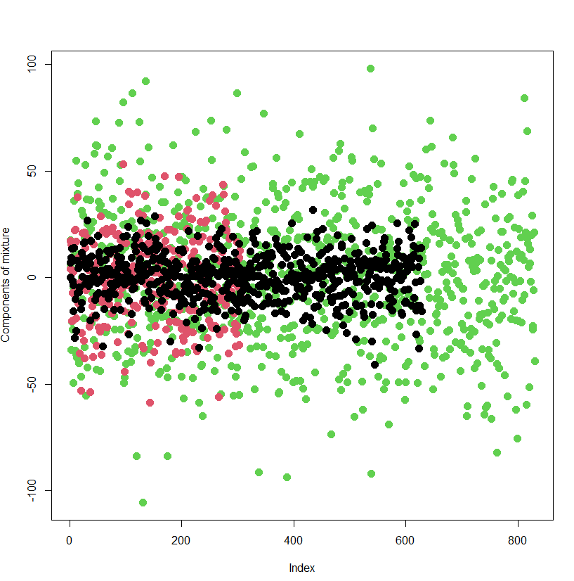
Before diving into the MCMC magic, the code begins by generating synthetic data. This dataset represents multiple groups, each with its own characteristics (such as coefficients and variances). These groups are modeled using different regression equations, with each group having a unique set of explanatory variables and associated parameters.
The key here is that the generated data is structured in a way that mimics real-world scenarios where multiple groups coexist, and the goal is to uncover the relationships between variables in each group. By using simulated data, we can apply MCMC methods and see how the model estimates parameters under controlled conditions.
The Power of MCMC: Estimating Model Parameters
Now, let’s talk about the core of this approach: Markov Chain Monte Carlo (MCMC). In essence, MCMC is a method for drawing samples from complex, high-dimensional probability distributions. In our case, we’re interested in the posterior distribution of the parameters in our mixture model — things like regression coefficients (betas) and variances (sigma). The mathematics of this approach has been discussed in detail in https://medium.com/towards-data-science/introduction-to-the-finite-normal-mixtures-in-regression-with-6a884810a692.
The MCMC process in the code is iterative, meaning that it refines its estimates over multiple cycles. Let’s break down how it works:
- Updating Group Labels: Given the current values of the model parameters, we begin by determining the most probable group membership for each observation. This is like assigning a “label” to each data point based on the current understanding of the model.
- Sampling Regression Coefficients (Betas): Next, we sample the regression coefficients for each group. These coefficients tell us how strongly the explanatory variables influence the dependent variable within each group.
- Sampling Variances (Sigma): We then update the variances (sigma) for each group. Variance is crucial as it tells us how spread out the data is within each group. Smaller variance means the data points are closely packed around the mean, while larger variance indicates more spread.
- Reordering Groups: Finally, we reorganize the groups based on the updated parameters, ensuring that the model can better fit the data. This helps in adjusting the model and improving its accuracy over time.
- Feature selection: It helps determine which variables are most relevant for each regression component. Using a probabilistic approach, it selects variables for each group based on their contribution to the model, with the inclusion probability calculated for each variable in the mixture model. This feature selection mechanism enables the model to focus on the most important predictors, improving both interpretability and performance. This idea has been discussed as a fully separate tool in https://medium.com/dev-genius/bayesian-variable-selection-for-linear-regression-based-on-stochastic-search-in-r-applicable-to-ml-5936d804ba4a . In the current implementation, I have combined it with mixture of regressions to make it powerful component of flexible regression framework. By sampling the inclusion probabilities during the MCMC process, the model can dynamically adjust which features are included, making it more flexible and capable of identifying the most impactful variables in complex datasets.
Once the algorithm has run through enough iterations, we can analyze the results. The code includes a simple visualization step that plots the estimated parameters, comparing them to the true values that were used to generate the synthetic data. This helps us understand how well the MCMC method has done in capturing the underlying structure of the data.
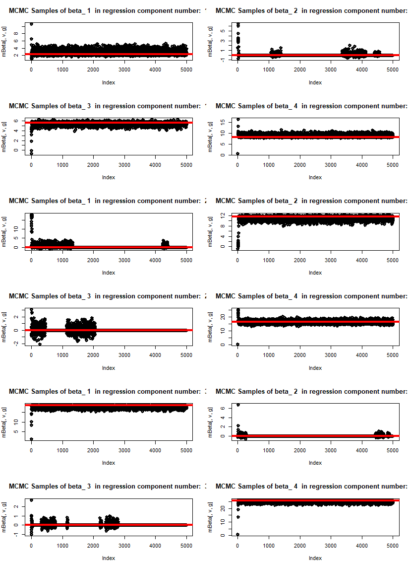
The graphs below present the outcome of the code with 5000 MCMC draws. We work with a mixture of three components, each with four potential explanatory variables. At the starting point we switch off some of the variables within individual mixtures. The algorithm is able to find only those features which have predictive power for the predicted variable. We plot the draws of individual beta parameters for all the components of regression. Some of them oscillate around 0. The red curve presents the true value of parameter beta in the data used for generating the mixture.
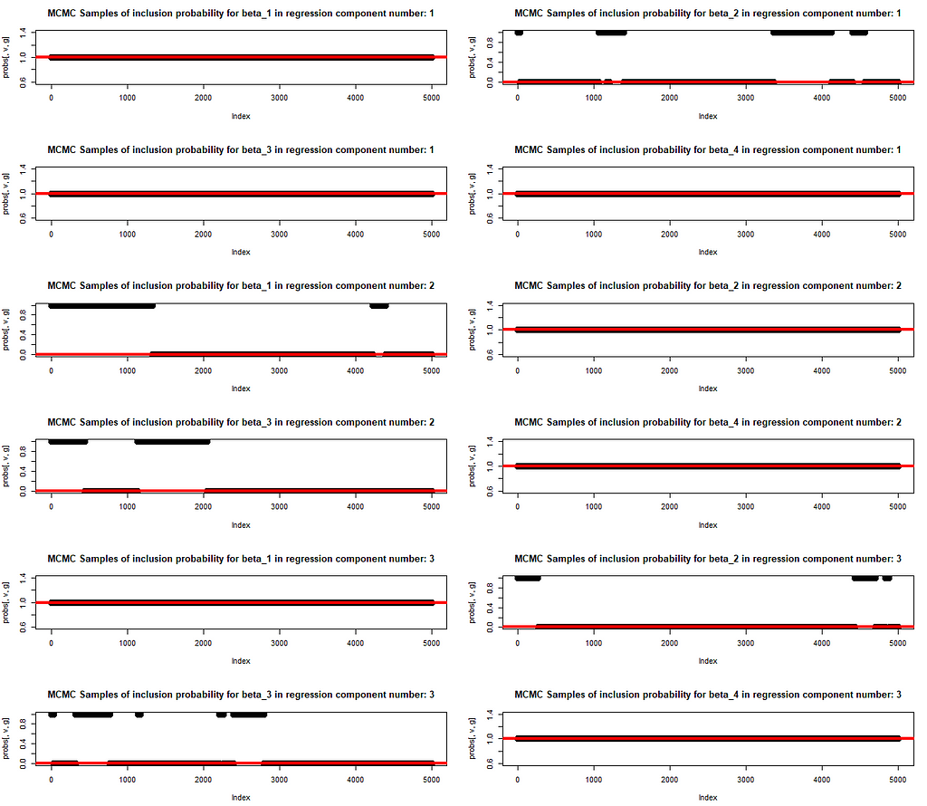
We also plot the MCMC draws of the inclusion probability. The red line at either 0 or 1 indicates if that parameter has been included in the original mixture of regression for generating the data. The learning of inclusion probability happens in parallel to the parameter training. This is exactly what allows for a trust in the trained values of betas. The model structure is revealed (i.e. the subset of variables with explanatory power is identified) and, at the same time, the correct values of beta are learnt.
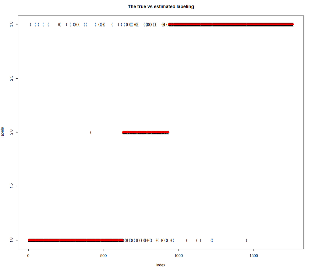
Finally, we present the outcome of classification of individual data points to the respective components of the mixture. The ability of the model to classify the data points to the component of the mixture they really stem from is great. The model has been wrong only in 6 % of cases.
Why This Is Interesting: The Power of Mixture Models in Action
What makes this approach particularly interesting is its ability to uncover hidden structures in data. Think about datasets that come from multiple sources or have inherent subpopulations, such as customer data, clinical trials, or even environmental measurements. Mixture models allow us to classify observations into these subpopulations without having to know their exact nature beforehand. The use of MCMC makes this even more powerful by allowing us to estimate parameters with high precision, even in cases where traditional estimation methods might fail.
Key Takeaways: Why MCMC and Mixture Models Matter
Mixture models with MCMC are incredibly powerful tools for analyzing complex datasets. By applying MCMC methods, we’re able to estimate parameters in situations where traditional models may struggle. This flexibility makes MCMC a go-to choice for many advanced data analysis tasks, from identifying customer segments to analyzing medical data or even predicting future trends based on historical patterns.
The code we explored in this article is just one example of how mixture models and MCMC can be applied in R. With some customization, you can apply these techniques to a wide variety of datasets, helping you uncover hidden insights and make more informed decisions.
For anyone interested in statistical modeling, machine learning, or data science, mastering mixture models and MCMC is a game-changer. These methods are versatile, powerful, and — when applied correctly — can unlock a wealth of insights from your data.
Final Thoughts
As data becomes increasingly complex, having the tools to model and interpret it effectively is more important than ever. Mixture models combined with MCMC offer a robust framework for handling multi-group data, and learning how to implement these techniques will significantly improve your analytical capabilities.
In the world of data science, mastering these advanced techniques opens up a vast array of possibilities, from business analytics to scientific research. With the R code provided, you now have a solid starting point for exploring mixture models and MCMC in your own projects, whether you’re uncovering hidden patterns in data or fine-tuning a predictive model. The next time you encounter a complex dataset, you’ll be well-equipped to dive deep and extract meaningful insights.
There is one important by product of the below implementation. Linear regression, while foundational in machine learning, often falls short in real-world applications due to its assumptions and limitations. One major issue is its assumption of a linear relationship between input features and the target variable, which rarely holds true in complex datasets.
Additionally, linear regression is sensitive to outliers and multicollinearity, where highly correlated features distort the model’s predictions. It also struggles with non-linear relationships and interactions between features, making it less flexible in capturing the complexity of modern data. In practice, data scientists often turn to more robust methods such as decision trees, random forests, support vector machines, and neural networks. These techniques can handle non-linearity, interactions, and large datasets more effectively, offering better predictive performance and adaptability in dynamic environments.
However, while above mentioned methods offer improved predictive power, they often come at the cost of interpretability. These models operate as “black boxes,” making it difficult to understand how input features are being transformed into predictions, which poses challenges for explain-ability and trust in critical decision-making applications.
So, is it possible to restore the shine of linear regression and make it a powerful tool again? Definitely, if you follow below implemented approach with the mixture of normal regression, you will feel the power of the underlying concept of linear regression with its great interpretability aspect!https://medium.com/media/5e3c113a30b77328ec5a3b91cd98a4d5/href
Unless otherwise noted, all images are by the author.
Integrating Feature Selection into the Model Estimation was originally published in Towards Data Science on Medium, where people are continuing the conversation by highlighting and responding to this story.


 Editor-Admin


