Detecting Anomalies in Social Media Volume Time Series
How I detect anomalies in social Media volumes: A Residual-Based ApproachPhoto by Joshua Hoehne on UnsplashIn the age of social media, analyzing conversation volumes has become crucial for understanding user behaviours, detecting trends, and, most importantly, identifying anomalies. Knowing when an anomaly is occurring can help management and marketing respond in crisis scenarios.In this article, we’ll explore a residual-based approach for detecting anomalies in social media volume time series data, using a real-world example from Twitter. For such a task, I am going to use data from Numenta Anomaly Benchmark, which provides volume data from Twitter posts with a 5-minute frame window amongst its benchmarks.We will analyze the data from two perspectives: as a first exercise we will detect anomalies using the full dataset, and then we will detect anomalies in a real-time scenario to check how responsive this method is.Detecting anomalies with the full datasetAnalyzing a Sample Twitter Volume DatasetLet’s start by loading and visualizing a sample Twitter volume dataset for Apple:Volume and log-Volume observed for AAPL Twitter volumesImage by AuthorFrom this plot, we can see that there are several spikes (anomalies) in our data. These spikes in volumes are the ones we want to identify.Looking at the second plot (log-scale) we can see that the Twitter volume data shows a clear daily cycle, with higher activity during the day and lower activity at night. This seasonal pattern is common in social media data, as it reflects the day-night activity of users. It also presents a weekly seasonality, but we will ignore it.Removing Seasonal TrendsWe want to make sure that this cycle does not interfere with our conclusions, thus we will remove it. To remove this seasonality, we’ll perform a seasonal decomposition.First, we’ll calculate the moving average (MA) of the volume, which will capture the trend. Then, we’ll compute the ratio of the observed volume to the MA, which gives us the multiplicative seasonal effect.Multiplicative effect of time on volumes Image by AuthorAs expected, the seasonal trend follows a day/night cycle with its peak during the day hours and its saddle at nighttime.To further proceed with the decomposition we need to calculate the expected value of the volume given the multiplicative trend found before.Volume and log-Volume observed and expected for AAPL Twitter volumesImage by AuthorAnalyzing Residuals and Detecting AnomaliesThe final component of the decomposition is the error resulting from the subtraction between the expected value and the true value. We can consider this measure as the de-meaned volume accounting for seasonality:Absolute Error and log-Error after seasonal decomposition of AAPL Twitter volumesImage by AuthorInterestingly, the residual distribution closely follows a Pareto distribution. This property allows us to use the Pareto distribution to set a threshold for detecting anomalies, as we can flag any residuals that fall above a certain percentile (e.g., 0.9995) as potential anomalies.Absolute Error and log-Error quantiles Vs Pareto quantilesImage by AuthorNow, I have to do a big disclaimer: this property I am talking about is not “True” per se. In my experience in social listening, I’ve observed that holds true with most social data. Except for some right skewness in a dataset with many anomalies.In this specific case, we have well over 15k observations, hence we will set the p-value at 0.9995. Given this threshold, roughly 5 anomalies for every 10.000 observations will be detected (assuming a perfect Pareto distribution).Therefore, if we check which observation in our data has an error whose p-value is higher than 0.9995, we get the following signals:Signals anomalies of AAPL Twitter volumesImage by AuthorFrom this graph, we see that the observations with the highest volumes are highlighted as anomalies. Of course, if we desire more or fewer signals, we can adjust the selected p-value, keeping in mind that, as it decreases, it will increase the number of signals.Real-Time Anomaly DetectionNow let’s switch to a real-time scenario. In this case, we will run the same algorithm for every new observation and check both which signals are returned and how quickly the signals are returned after the observation takes place:Live Signals of AAPL Twitter volumesImage by AuthorWe can clearly see that this time, we have more signals. This is justified as the Pareto curve we fit changes as the data at our disposal changes. The first three signals can be considered anomalies if we check the data up to “2015–03–08” but these are less important if we consider the entire dataset.By construction, the code provided returns with a signal limiting itself to the previous 24 hours. However, as we can see below, most of the signals are returned as soon as the new observation is considered, with a few exceptions already bolded:New signal at datetime 2015-03-03 21:02:53, relative to timestamp 2015-03-03

How I detect anomalies in social Media volumes: A Residual-Based Approach

In the age of social media, analyzing conversation volumes has become crucial for understanding user behaviours, detecting trends, and, most importantly, identifying anomalies. Knowing when an anomaly is occurring can help management and marketing respond in crisis scenarios.
In this article, we’ll explore a residual-based approach for detecting anomalies in social media volume time series data, using a real-world example from Twitter. For such a task, I am going to use data from Numenta Anomaly Benchmark, which provides volume data from Twitter posts with a 5-minute frame window amongst its benchmarks.
We will analyze the data from two perspectives: as a first exercise we will detect anomalies using the full dataset, and then we will detect anomalies in a real-time scenario to check how responsive this method is.
Detecting anomalies with the full dataset
Analyzing a Sample Twitter Volume Dataset
Let’s start by loading and visualizing a sample Twitter volume dataset for Apple: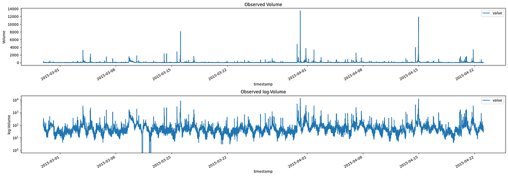
Image by Author
From this plot, we can see that there are several spikes (anomalies) in our data. These spikes in volumes are the ones we want to identify.
Looking at the second plot (log-scale) we can see that the Twitter volume data shows a clear daily cycle, with higher activity during the day and lower activity at night. This seasonal pattern is common in social media data, as it reflects the day-night activity of users. It also presents a weekly seasonality, but we will ignore it.
Removing Seasonal Trends
We want to make sure that this cycle does not interfere with our conclusions, thus we will remove it. To remove this seasonality, we’ll perform a seasonal decomposition.
First, we’ll calculate the moving average (MA) of the volume, which will capture the trend. Then, we’ll compute the ratio of the observed volume to the MA, which gives us the multiplicative seasonal effect.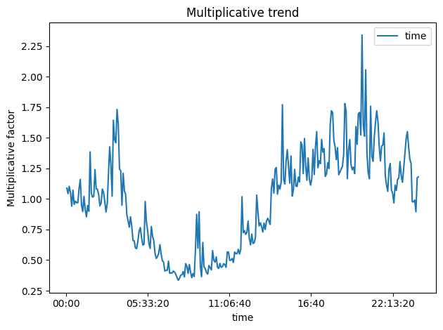
Image by Author
As expected, the seasonal trend follows a day/night cycle with its peak during the day hours and its saddle at nighttime.
To further proceed with the decomposition we need to calculate the expected value of the volume given the multiplicative trend found before.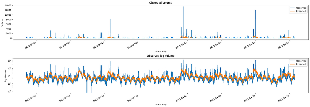
Image by Author
Analyzing Residuals and Detecting Anomalies
The final component of the decomposition is the error resulting from the subtraction between the expected value and the true value. We can consider this measure as the de-meaned volume accounting for seasonality: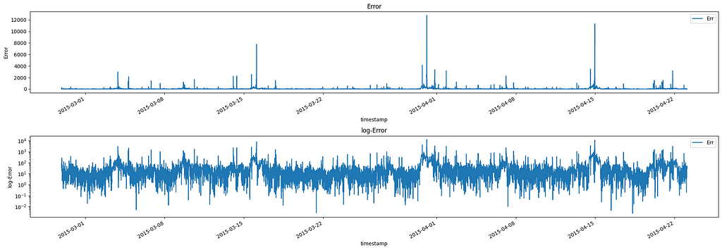
Image by Author
Interestingly, the residual distribution closely follows a Pareto distribution. This property allows us to use the Pareto distribution to set a threshold for detecting anomalies, as we can flag any residuals that fall above a certain percentile (e.g., 0.9995) as potential anomalies.
Image by Author
Now, I have to do a big disclaimer: this property I am talking about is not “True” per se. In my experience in social listening, I’ve observed that holds true with most social data. Except for some right skewness in a dataset with many anomalies.
In this specific case, we have well over 15k observations, hence we will set the p-value at 0.9995. Given this threshold, roughly 5 anomalies for every 10.000 observations will be detected (assuming a perfect Pareto distribution).
Therefore, if we check which observation in our data has an error whose p-value is higher than 0.9995, we get the following signals: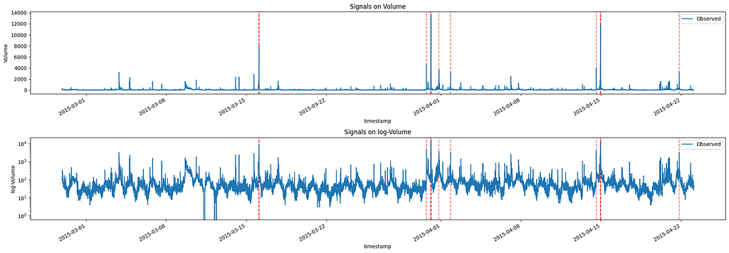
Image by Author
From this graph, we see that the observations with the highest volumes are highlighted as anomalies. Of course, if we desire more or fewer signals, we can adjust the selected p-value, keeping in mind that, as it decreases, it will increase the number of signals.
Real-Time Anomaly Detection
Now let’s switch to a real-time scenario. In this case, we will run the same algorithm for every new observation and check both which signals are returned and how quickly the signals are returned after the observation takes place: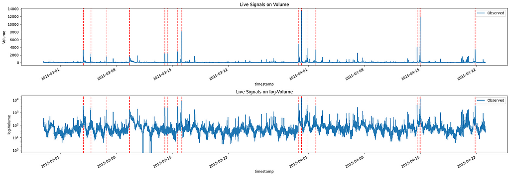
Image by Author
We can clearly see that this time, we have more signals. This is justified as the Pareto curve we fit changes as the data at our disposal changes. The first three signals can be considered anomalies if we check the data up to “2015–03–08” but these are less important if we consider the entire dataset.
By construction, the code provided returns with a signal limiting itself to the previous 24 hours. However, as we can see below, most of the signals are returned as soon as the new observation is considered, with a few exceptions already bolded:
New signal at datetime 2015-03-03 21:02:53, relative to timestamp 2015-03-03 21:02:53
New signal at datetime 2015-03-03 21:07:53, relative to timestamp 2015-03-03 21:07:53
New signal at datetime 2015-03-03 21:12:53, relative to timestamp 2015-03-03 21:12:53
New signal at datetime 2015-03-03 21:17:53, relative to timestamp 2015-03-03 21:17:53 **
New signal at datetime 2015-03-05 05:37:53, relative to timestamp 2015-03-04 20:07:53
New signal at datetime 2015-03-07 09:47:53, relative to timestamp 2015-03-06 19:42:53 **
New signal at datetime 2015-03-09 15:57:53, relative to timestamp 2015-03-09 15:57:53
New signal at datetime 2015-03-09 16:02:53, relative to timestamp 2015-03-09 16:02:53
New signal at datetime 2015-03-09 16:07:53, relative to timestamp 2015-03-09 16:07:53
New signal at datetime 2015-03-14 01:37:53, relative to timestamp 2015-03-14 01:37:53
New signal at datetime 2015-03-14 08:52:53, relative to timestamp 2015-03-14 08:52:53
New signal at datetime 2015-03-14 09:02:53, relative to timestamp 2015-03-14 09:02:53
New signal at datetime 2015-03-15 16:12:53, relative to timestamp 2015-03-15 16:12:53
New signal at datetime 2015-03-16 02:52:53, relative to timestamp 2015-03-16 02:52:53
New signal at datetime 2015-03-16 02:57:53, relative to timestamp 2015-03-16 02:57:53
New signal at datetime 2015-03-16 03:02:53, relative to timestamp 2015-03-16 03:02:53
New signal at datetime 2015-03-30 17:57:53, relative to timestamp 2015-03-30 17:57:53
New signal at datetime 2015-03-30 18:02:53, relative to timestamp 2015-03-30 18:02:53
New signal at datetime 2015-03-31 03:02:53, relative to timestamp 2015-03-31 03:02:53
New signal at datetime 2015-03-31 03:07:53, relative to timestamp 2015-03-31 03:07:53
New signal at datetime 2015-03-31 03:12:53, relative to timestamp 2015-03-31 03:12:53
New signal at datetime 2015-03-31 03:17:53, relative to timestamp 2015-03-31 03:17:53
New signal at datetime 2015-03-31 03:22:53, relative to timestamp 2015-03-31 03:22:53
New signal at datetime 2015-03-31 03:27:53, relative to timestamp 2015-03-31 03:27:53
New signal at datetime 2015-03-31 03:32:53, relative to timestamp 2015-03-31 03:32:53
New signal at datetime 2015-03-31 03:37:53, relative to timestamp 2015-03-31 03:37:53
New signal at datetime 2015-03-31 03:42:53, relative to timestamp 2015-03-31 03:42:53
New signal at datetime 2015-03-31 20:22:53, relative to timestamp 2015-03-31 20:22:53 **
New signal at datetime 2015-04-02 12:52:53, relative to timestamp 2015-04-01 20:42:53 **
New signal at datetime 2015-04-14 14:12:53, relative to timestamp 2015-04-14 14:12:53
New signal at datetime 2015-04-14 22:52:53, relative to timestamp 2015-04-14 22:52:53
New signal at datetime 2015-04-14 22:57:53, relative to timestamp 2015-04-14 22:57:53
New signal at datetime 2015-04-14 23:02:53, relative to timestamp 2015-04-14 23:02:53
New signal at datetime 2015-04-14 23:07:53, relative to timestamp 2015-04-14 23:07:53
New signal at datetime 2015-04-14 23:12:53, relative to timestamp 2015-04-14 23:12:53
New signal at datetime 2015-04-14 23:17:53, relative to timestamp 2015-04-14 23:17:53
New signal at datetime 2015-04-14 23:22:53, relative to timestamp 2015-04-14 23:22:53
New signal at datetime 2015-04-14 23:27:53, relative to timestamp 2015-04-14 23:27:53
New signal at datetime 2015-04-21 20:12:53, relative to timestamp 2015-04-21 20:12:53
As we can see, the algorithm is able to detect anomalies in real time, with most signals being raised as soon as the new observation is considered. This allows organizations to respond quickly to unexpected changes in social media conversation volumes.
Conclusions and Further Improvements
The residual-based approach presented in this article provides a responsive tool for detecting anomalies in social media volume time series. This method can help companies and marketers identify important events, trends, and potential crises as they happen.
While this algorithm is already effective, there are several points that can be further developed, such as:
- Dependence on a fixed window for real-time detection, as for now depends on all previous data
- Exploring different time granularities (e.g., hourly instead of 5-minute intervals)
- Validating the Pareto distribution assumption using statistical tests
- …
Please leave some claps if you enjoyed the article and feel free to comment, any suggestion and feedback is appreciated!
Here you can find a notebook with an implementation.
Detecting Anomalies in Social Media Volume Time Series was originally published in Towards Data Science on Medium, where people are continuing the conversation by highlighting and responding to this story.


 Editor-Admin


