
Support Vector Machines: A Progression of Algorithms
MMC, SVC, SVM: What’s the difference?The Support Vector Machine (SVM) is a popular learning algorithm used for many classification problems. They are known to be useful out-of-the-box (not much manual configuration required), and they are valuable for applications where knowledge of the class boundaries is more important than knowledge of the class distributions.When working with SVMs, you may hear people mention Support Vector Classifiers (SVC) or Maximal Margin Classifiers (MMC). While these algorithms are all related, there is an important distinction to be made between the three of them.To fully understand SVMs, we must appreciate the progression of the following algorithms, ordered from lowest to highest complexity:Maximal Margin Classifier (MMC) -> Support Vector Classifier (SVC) -> Support Vector Machine (SVM)In this progression, each algorithm extends upon the functionality of the previous that allows it to find a decision boundary that is increasingly more flexible and/or robust. Understanding this progression will allow us to fully appreciate the power of Support Vector Machines.ContentsMaximal Margin ClassifierSupport Vector ClassifierSupport Vector MachineTLDRSourcesMaximal Margin ClassifierLet’s start by considering the following problem.Suppose we’re dealing with some data that consists of observations that fall into one of two classes, and these classes are linearly separable (i.e. we can define a line that separates the class distributions). How do we define the decision boundary that “best” separates these classes?A few (of the many) possible hyperplanes that completely separate the observation classes (highlighted in green & blue). Image by authorFrom the picture above, we can notice the following:If data is linearly separable, there exist multiple (infinite!) hyperplanes which can separate the classes.However, it seems that some hyperplanes are better approximators of the true decision boundary that separates these classes.How do we choose one?Enter the Maximal Margin Classifier, the most basic of the three algorithms. At a very high level, the MMC finds the decision boundary that satisfies the following:Find the widest “slab” that can fit between the two observation classes.Define the decision boundary as the line that cuts that slab in half.Essentially, the goal is to find the boundary such that the distance between the observation classes & the decision boundary is maximized. In this case, distance is defined as the perpendicular distance between an observation & the decision boundary. The smallest such distance is called the margin.More formally, the MMC finds the boundary that solves the following optimization problem:MMC optimization problem. Image by author, inspired by An Introduction to Statistical Learning, Chapter 9Line by line translation:Maximize the margin M,Such that the sum of the squared coefficients of the hyperplane sum up to 1,And every observation is at least distance M away from the hyperplane, on the appropriate side of the boundary.Satisfying the constraint in 1 guarantees that the distance between any observation and the hyperplane is defined by the equation in 2. This can be shown by plugging the constraint into the standard equation for computing the distance between a point to a plane shown below.Distance from point to plane. Image by author, inspired by An Introduction to Statistical Learning, Chapter 9Satisfying constraint 2 of the MMC optimization problem would result in the denominator of the equation above equaling 1, which leaves us with constraint 3 (keep in mind that y = -1 or 1 for every observation).The logic of the MMC is intuitive & simple, but the MMC doesn’t end up being very useful in practice. Very rarely do we deal with data that is perfectly linearly separable as it exists in its current dimension space.In this dimension space, there exists no linear boundary that perfectly separates the observation classes (i.e. no MMC exists). Image by authorAdditionally, even when we are dealing with perfectly linearly separable data, the boundary defined by the MMC may be suboptimal.Consider the data below:Solid red: the decision boundary computed by the MMC. Solid black: an imperfect (but possibly better?) decision boundary for distinguishing the observation classes. Image by authorThe decision boundary computed by the MMC is highlighted in solid red. Since the MMC must perfectly separate the observations, the boundary it produces is highly sensitive to individual values. Consider the blue observation circled in purple in the image above. Removal of that single point would result in a MMC boundary that is much closer to the boundary defined by the solid black line. This high sensitivity to individual observations means the MMC has high variance, which is not ideal for maximizing its ability to classify future unseen observations.So, how can we extend the MMC to cope with these limitations?Support Vector ClassifierEnter the Support Vector Classifier (SVC).
 Editor-Admin
MMC, SVC, SVM: What’s the difference?
The Support Vector Machine (SVM) is a popular learning algorithm used for many classification problems. They are known to be useful out-of-the-box (not much manual configuration required), and they are valuable for applications where knowledge of the class boundaries is more important than knowledge of the class distributions.
When working with SVMs, you may hear people mention Support Vector Classifiers (SVC) or Maximal Margin Classifiers (MMC). While these algorithms are all related, there is an important distinction to be made between the three of them.
To fully understand SVMs, we must appreciate the progression of the following algorithms, ordered from lowest to highest complexity:
- Maximal Margin Classifier (MMC) -> Support Vector Classifier (SVC) -> Support Vector Machine (SVM)
In this progression, each algorithm extends upon the functionality of the previous that allows it to find a decision boundary that is increasingly more flexible and/or robust. Understanding this progression will allow us to fully appreciate the power of Support Vector Machines.
Contents
- Maximal Margin Classifier
- Support Vector Classifier
- Support Vector Machine
- TLDR
- Sources
Maximal Margin Classifier
Let’s start by considering the following problem.
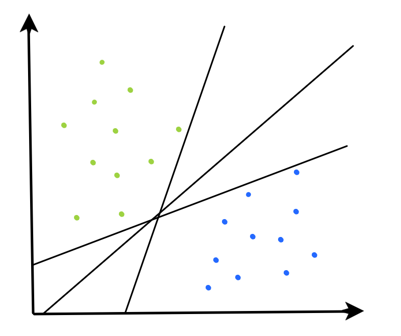
Suppose we’re dealing with some data that consists of observations that fall into one of two classes, and these classes are linearly separable (i.e. we can define a line that separates the class distributions). How do we define the decision boundary that “best” separates these classes?
From the picture above, we can notice the following:
- If data is linearly separable, there exist multiple (infinite!) hyperplanes which can separate the classes.
- However, it seems that some hyperplanes are better approximators of the true decision boundary that separates these classes.
How do we choose one?
Enter the Maximal Margin Classifier, the most basic of the three algorithms. At a very high level, the MMC finds the decision boundary that satisfies the following:
- Find the widest “slab” that can fit between the two observation classes.
- Define the decision boundary as the line that cuts that slab in half.
Essentially, the goal is to find the boundary such that the distance between the observation classes & the decision boundary is maximized. In this case, distance is defined as the perpendicular distance between an observation & the decision boundary. The smallest such distance is called the margin.
More formally, the MMC finds the boundary that solves the following optimization problem: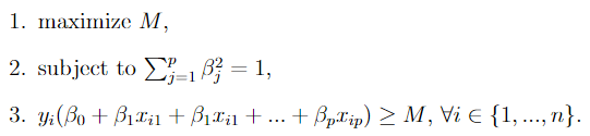
Line by line translation:
- Maximize the margin M,
- Such that the sum of the squared coefficients of the hyperplane sum up to 1,
- And every observation is at least distance M away from the hyperplane, on the appropriate side of the boundary.
Satisfying the constraint in 1 guarantees that the distance between any observation and the hyperplane is defined by the equation in 2. This can be shown by plugging the constraint into the standard equation for computing the distance between a point to a plane shown below.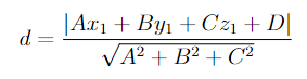
Satisfying constraint 2 of the MMC optimization problem would result in the denominator of the equation above equaling 1, which leaves us with constraint 3 (keep in mind that y = -1 or 1 for every observation).
The logic of the MMC is intuitive & simple, but the MMC doesn’t end up being very useful in practice. Very rarely do we deal with data that is perfectly linearly separable as it exists in its current dimension space.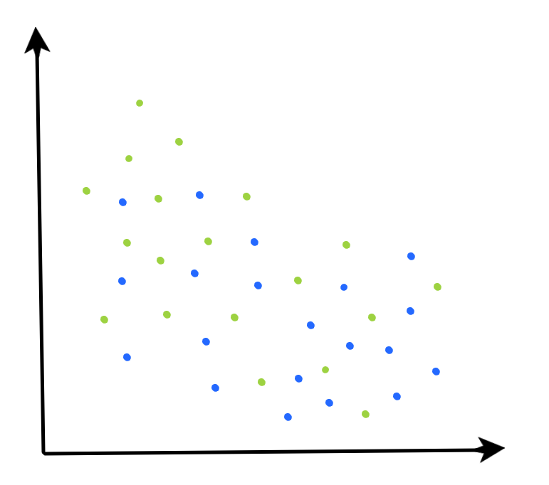
Additionally, even when we are dealing with perfectly linearly separable data, the boundary defined by the MMC may be suboptimal.
Consider the data below: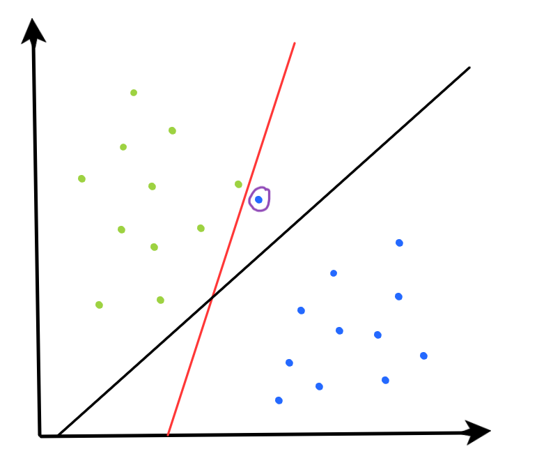
The decision boundary computed by the MMC is highlighted in solid red. Since the MMC must perfectly separate the observations, the boundary it produces is highly sensitive to individual values. Consider the blue observation circled in purple in the image above. Removal of that single point would result in a MMC boundary that is much closer to the boundary defined by the solid black line. This high sensitivity to individual observations means the MMC has high variance, which is not ideal for maximizing its ability to classify future unseen observations.
So, how can we extend the MMC to cope with these limitations?
Support Vector Classifier
Enter the Support Vector Classifier (SVC).
The SVC algorithm (also known as the soft margin classifier) is an extension of the MMC algorithm that includes an additional “budget” parameter to quantify how much misclassification error to tolerate.
Having a budget for misclassification error is useful for the following reasons we previously mentioned:
- Most data you’ll deal with will not be perfectly linearly separable, so a MMC won’t exist.
- The MMC is highly sensitive to individual observations, so atypical values may lead to the MMC finding a suboptimal decision boundary that generalizes poorly to unseen data.
Formally, the SVC computes the decision boundary that solves the following optimization problem.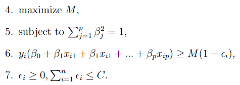
It is very similar to the MMC optimization problem we saw previously. The key differences are:
- C is the non-negative parameter that quantifies how much misclassification error to tolerate. The constraint introduced in 7 specifies that the sum of the misclassification errors across all observations the classifier is fit on must be bounded by this value.
- Constraint 6 is similar to constraint 3 we saw in the MMC optimization problem, but adjusted to account for the fact that not all observations will be on the correct side of the margin (or the hyperplane).
Notice that the MMC optimization problem is a special case of the SVC optimization problem where C = 0.
Additionally, the decision boundaries computed by the MMC & SVC only depend on the observations that lie on or violate the margin. These are known as the support vectors.
Typically, the ideal value of C is determined via cross validation. Tuning the C parameter impacts the bias-variance tradeoff of the classifier in the following manner:
- Large C -> more observations will lie on/violate the margin, so the classifier is dependent on more datapoints (more support vectors). Thus, the classifier will have lower variance.
- Small C -> resulting classifier will be closer to an MMC, so less observations will lie on/violate the margin. This implies higher sensitivity to individual observations, which implies higher variance.
It’s important to note that the effect of varying C as described above is specific to the optimization problem depicted in the picture. In practice, the effect of varying the C parameter may be reversed in some library implementations of the SVC (ex: scikit-learn’s SVC) as we’ll see below.
Let’s look at a concrete example of the effect that varying C has on the final classifier.
import matplotlib.pyplot as plt
import numpy as np
from sklearn.datasets import make_blobs
from sklearn import svm

# create 100 separable points
X, Y = make_blobs(n_samples=100, centers=2, random_state=0, cluster_std=0.60)

# regularization parameter -> smaller values = higher misclassification tolerance
C_list = [0.05, 0.5, 1]

fignum = 1

for c_val in C_list:
  # fit the model
  clf = svm.SVC(kernel="linear", C=c_val)
  clf.fit(X, Y)

  # plot the line, the points, and the nearest vectors to the plane
  xx = np.linspace(-1, 5, 10)
  yy = np.linspace(-1, 5, 10)

  X1, X2 = np.meshgrid(xx, yy)
  Z = np.empty(X1.shape)
  for (i, j), val in np.ndenumerate(X1):
      x1 = val
      x2 = X2[i, j]
      p = clf.decision_function([[x1, x2]])
      Z[i, j] = p[0]
  levels = [-1.0, 0.0, 1.0]
  linestyles = ["dashed", "solid", "dashed"]
  colors = "k"
  plt.figure(fignum, figsize=(4,3))
  plt.contour(X1, X2, Z, levels, colors=colors, linestyles=linestyles)

  #highlight support vectors
  plt.scatter(
          clf.support_vectors_[:, 0],
          clf.support_vectors_[:, 1],
          s=80,
          facecolors="none",
          zorder=10,
          edgecolors="k",
          cmap=plt.get_cmap("RdBu"),
      )

  plt.scatter(X[:, 0], X[:, 1], c=Y, cmap=plt.cm.Paired, edgecolor="black", s=20)
  plt.title(f"C = {c_val}")
  plt.axis("tight")
  fignum = fignum + 1

plt.show()
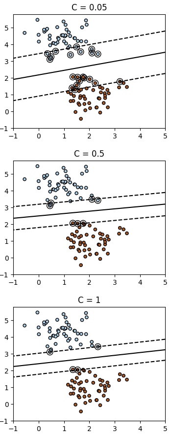
The example above uses scikit-learn’s SVC implementation, where the “strength of the regularization is inversely proportional to C”. So, smaller values of C are associated with a higher misclassification “budget”.
The visuals reinforce what we stated above: classifiers fit with higher tolerance for misclassification errors will have more support vectors (indicated by the circled observations) i.e. more observations will lie on or violate the margin. Since a larger portion of the data will play a role in the classifier fit, it will inevitably lead to the classifier being less sensitive to individual changes in data (i.e. less variance from dataset to dataset).
However, the SVC is limited as it can only define a linear decision boundary in the feature space, which may be suboptimal when working with more complex datasets.
Consider the following example.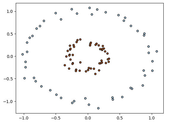
It’s pretty clear that any linear boundary we attempt to define here will do a poor job at approximating the true boundary that separates the observation classes. Let’s look at the Support Vector Machine (SVM), which is an extension of the SVC that allows us to produce decision boundaries that can fit to non-linearly separable data.
Support Vector Machine
In general, there are two strategies that are commonly used when trying to classify non-linear data:
- Fit a non-linear classification algorithm to the data in its original feature space.
- Enlarge the feature space to a higher dimension where a linear decision boundary exists.
SVMs aim to find a linear decision boundary in a higher dimensional space, but they do this in a computationally efficient manner using Kernel functions, which allow them to find this decision boundary without having to apply the non-linear transformation to the observations.
There exist many different options to enlarge the feature space via some non-linear transformation of features (higher order polynomial, interaction terms, etc.). Let’s look at an example where we expand the feature space by applying a quadratic polynomial expansion.
Suppose our original feature set consists of the p features below.
Our new feature set after applying the quadratic polynomial expansion consists of the 2p features below.
Now, we need to solve the following optimization problem.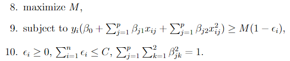
It’s the same as the SVC optimization problem we saw earlier, but now we have quadratic terms included in our feature space, so we have twice as many features. The solution to the above will be linear in the quadratic space, but non-linear when translated back to the original feature space.
However, to solve the problem above, it would require applying the quadratic polynomial transformation to every observation the SVC would be fit on. This could be computationally expensive with high dimensional data. Additionally, for more complex data, a linear decision boundary may not exist even after applying the quadratic expansion. In that case, we must explore other higher dimensional spaces before we can find a linear decision boundary, where the cost of applying the non-linear transformation to our data could be very computationally expensive. Ideally, we would be able to find this decision boundary in the higher dimensional space without having to apply the required non-linear transformation to our data.
Luckily, it turns out that the solution to the SVC optimization problem above does not require explicit knowledge of the feature vectors for the observations in our dataset. We only need to know how the observations compare to each other in the higher dimensional space. In mathematical terms, this means we just need to compute the pairwise inner products (chap. 2 here explains this in detail), where the inner product can be thought of as some value that quantifies the similarity of two observations.
It turns out for some feature spaces, there exists functions (i.e. Kernel functions) that allow us to compute the inner product of two observations without having to explicitly transform those observations to that feature space. More detail behind this Kernel magic and when this is possible can be found in chap. 3 & chap. 6 here.
Since these Kernel functions allow us to operate in a higher dimensional space, we have the freedom to define decision boundaries that are much more flexible than that produced by a typical SVC.
Let’s look at a popular Kernel function: the Radial Basis Function (RBF) Kernel.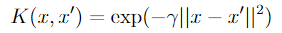
The formula is shown above for reference, but for the sake of basic intuition the details aren’t important: just think of it as something that quantifies how “similar” two observations are in a high (infinite!) dimensional space.
Let’s revisit the data we saw at the end of the SVC section. When we apply the RBF kernel to an SVM classifier & fit it to that data, we can produce a decision boundary that does a much better job of distinguishing the observation classes than that of the SVC.
import matplotlib.pyplot as plt
import numpy as np
from sklearn.datasets import make_circles
from sklearn import svm

# create circle within a circle
X, Y = make_circles(n_samples=100, factor=0.3, noise=0.05, random_state=0)

kernel_list = ['linear','rbf']

fignum = 1

for k in kernel_list:
  # fit the model
  clf = svm.SVC(kernel=k, C=1)
  clf.fit(X, Y)

  # plot the line, the points, and the nearest vectors to the plane
  xx = np.linspace(-2, 2, 8)
  yy = np.linspace(-2, 2, 8)

  X1, X2 = np.meshgrid(xx, yy)
  Z = np.empty(X1.shape)
  for (i, j), val in np.ndenumerate(X1):
      x1 = val
      x2 = X2[i, j]
      p = clf.decision_function([[x1, x2]])
      Z[i, j] = p[0]
  levels = [-1.0, 0.0, 1.0]
  linestyles = ["dashed", "solid", "dashed"]
  colors = "k"
  plt.figure(fignum, figsize=(4,3))
  plt.contour(X1, X2, Z, levels, colors=colors, linestyles=linestyles)
  plt.scatter(
          clf.support_vectors_[:, 0],
          clf.support_vectors_[:, 1],
          s=80,
          facecolors="none",
          zorder=10,
          edgecolors="k",
          cmap=plt.get_cmap("RdBu"),
      )
  plt.scatter(X[:, 0], X[:, 1], c=Y, cmap=plt.cm.Paired, edgecolor="black", s=20)

  # print kernel & corresponding accuracy score
  plt.title(f"Kernel = {k}: Accuracy = {clf.score(X, Y)}")

  plt.axis("tight")
  fignum = fignum + 1

plt.show()
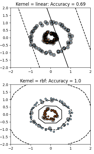
Ultimately, there are many different choices for Kernel functions, which provides lots of freedom in what kinds of decision boundaries we can produce. This can be very powerful, but it’s important to keep in mind to accompany these Kernel functions with appropriate regularization to reduce chances of overfitting.
TLDR
If you made it this far, I hope you enjoyed the overview of the progression of the three algorithms. Hopefully you acquired some appreciation for the power of Support Vector Machines along the way. If there are any details I missed or was incorrect about, I’d love to hear it in the comments.
In summary:
- MMC: simple & intuitive classifier that can be effective when there is a clear linear distinction in class boundaries.
- SVC: effective when data is not perfectly linearly separable, but class boundaries can still be approximated well in a linear fashion.
- SVM: effective for finding complex, non-linear class boundaries in a computationally efficient manner.
Check out the sources listed below if you’re interested in learning more.
Sources
Basic Overview:
- Introduction to Statistical Learning (Chapter 9)
Bias-Variance:
Datasets:
- https://scikit-learn.org/stable/datasets/sample_generators.html#generators-for-classification-and-clustering
- https://scikit-learn.org/stable/api/sklearn.datasets.html
Technical explanation of SVMs & Kernel Theory:
- https://people.cs.umass.edu/~domke/courses/sml2011/07kernels.pdf -> highly recommend
- https://www.reddit.com/r/MachineLearning/comments/1joh9v/can_someone_explain_kernel_trick_intuitively/
- The Elements of Statistical Learning (Chapter 12.3)
Simple & intuitive videos:
Support Vector Machines: A Progression of Algorithms was originally published in Towards Data Science on Medium, where people are continuing the conversation by highlighting and responding to this story.