A Derivation and Application of Restricted Boltzmann Machines (2024 Nobel Prize)
Investigating Geoffrey Hinton’s Nobel Prize-winning work and building it from scratch using PyTorchOne recipient of the 2024 Nobel Prize in Physics was Geoffrey Hinton for his contributions in the field of AI and machine learning. A lot of people know he worked on neural networks and is termed the “Godfather of AI”, but few understand his works. In particular, he pioneered Restricted Boltzmann Machines (RBMs) decades ago.This article is going to be a walkthrough of RBMs and will hopefully provide some intuition behind these complex mathematical machines. I will provide some code on implementing RBMs from scratch in PyTorch after going through the derivations.An Overview of RBMsRBMs are a form of unsupervised learning (only the inputs are used to learn- no output labels are used). This means we can automatically extract meaningful features in the data without relying on outputs. An RBM is a network with two different types of neurons with binary inputs: visible, x, and hidden, h. Visible neurons take in the input data and hidden neurons learn to detect features/patterns.RBM with input x and hidden layer y. Source: [1]In more technical terms, we say an RBM is an undirected bipartite graphical model with stochastic binary visible and hidden variables. The main goal of an RBM is to minimize the energy of the joint configuration E(x,h) often using contrastive learning (discussed later on).What is Energy?An energy function doesn’t correspond to physical energy, but it does come from physics/statistics. Think of it like a scoring function. An energy function E assigns lower scores (energies) to configurations x that we want our model to prefer, and higher scores to configurations we want it to avoid. The energy function is something we get to choose as model designers.For RBMs, the energy function is as follows (modeled after the Boltzmann distribution):RBM energy function. Source: AuthorThe energy function consists of 3 terms. The first one is the interaction between the hidden and visible layer with weights, W. The second is the sum of the bias terms for the visible units. The third is the sum of the bias terms for the hidden units.Probability DistributionWith the energy function, we can calculate the probability of the joint configuration given by the Boltzmann distribution. With this probability function, we can model our units:Probability for joint configuration for RBMs. Source: AuthorZ is the partition function (also known as the normalization constant). It is the sum of e^(-E) over all possible configurations of visible and hidden units. The big challenge with Z is that it’s typically computationally intractable to calculate exactly because you need to sum over all possible configurations of v and h. For example, with binary units, if you have m visible units and n hidden units, you need to sum over 2^(m+n) configurations. Therefore, we need a way to avoid calculating Z.InferenceWith those functions and distributions defined, we can go over some derivations for inference before talking about training and implementation. We already mentioned the inability to calculate Z in the joint probability distribution. To get around this, we can use Gibbs Sampling. Gibbs Sampling is a Markov Chain Monte Carlo algorithm for sampling from a specified multivariate probability distribution when direct sampling from the joint distribution is difficult, but sampling from the conditional distribution is more practical [2]. Therefore, we need conditional distributions.The great part about a restricted Boltzmann versus a fully connected Boltzmann is the fact that there are no connections within layers. This means given the visible layer, all hidden units are conditionally independent and vice versa. Let’s look at what that simplifies down to starting with p(x|h):Conditional distribution p(h|x). Source: AuthorWe can see the conditional distribution simplifies down to a sigmoid function where j is the jᵗʰ row of W. There is a far more rigorous calculation I have included in the appendix proving the first line of this derivation. Reach out if interested! Let’s now observe the conditional distribution p(h|x):Conditional distribution p(x|h). Source: AuthorWe can see this conditional distribution also simplifies down to a sigmoid function where k is the kᵗʰ row of W. Because of the restricted criteria in the RBM, the conditional distributions simplify to easy computations for Gibbs Sampling during inference. Once we understand what exactly the RBM is trying to learn, we will implement this in PyTorch.Model LearningAs with most of deep learning, we are trying to minimize the negative log-likelihood (NLL) to train our model. For the RBM:NLL for RBM. Source: AuthorTaking the derivative of this yields:Derivative of NLL. Source: AuthorThe first term on the left-hand side of the equation is called positive phase because it pushes the model to lower the energy of real data. This term involves taking the expectation over hidden units h give

Investigating Geoffrey Hinton’s Nobel Prize-winning work and building it from scratch using PyTorch
One recipient of the 2024 Nobel Prize in Physics was Geoffrey Hinton for his contributions in the field of AI and machine learning. A lot of people know he worked on neural networks and is termed the “Godfather of AI”, but few understand his works. In particular, he pioneered Restricted Boltzmann Machines (RBMs) decades ago.
This article is going to be a walkthrough of RBMs and will hopefully provide some intuition behind these complex mathematical machines. I will provide some code on implementing RBMs from scratch in PyTorch after going through the derivations.
An Overview of RBMs
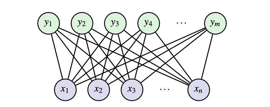
RBMs are a form of unsupervised learning (only the inputs are used to learn- no output labels are used). This means we can automatically extract meaningful features in the data without relying on outputs. An RBM is a network with two different types of neurons with binary inputs: visible, x, and hidden, h. Visible neurons take in the input data and hidden neurons learn to detect features/patterns.
In more technical terms, we say an RBM is an undirected bipartite graphical model with stochastic binary visible and hidden variables. The main goal of an RBM is to minimize the energy of the joint configuration E(x,h) often using contrastive learning (discussed later on).
What is Energy?
An energy function doesn’t correspond to physical energy, but it does come from physics/statistics. Think of it like a scoring function. An energy function E assigns lower scores (energies) to configurations x that we want our model to prefer, and higher scores to configurations we want it to avoid. The energy function is something we get to choose as model designers.
For RBMs, the energy function is as follows (modeled after the Boltzmann distribution):
The energy function consists of 3 terms. The first one is the interaction between the hidden and visible layer with weights, W. The second is the sum of the bias terms for the visible units. The third is the sum of the bias terms for the hidden units.
Probability Distribution
With the energy function, we can calculate the probability of the joint configuration given by the Boltzmann distribution. With this probability function, we can model our units:
Z is the partition function (also known as the normalization constant). It is the sum of e^(-E) over all possible configurations of visible and hidden units. The big challenge with Z is that it’s typically computationally intractable to calculate exactly because you need to sum over all possible configurations of v and h. For example, with binary units, if you have m visible units and n hidden units, you need to sum over 2^(m+n) configurations. Therefore, we need a way to avoid calculating Z.
Inference
With those functions and distributions defined, we can go over some derivations for inference before talking about training and implementation. We already mentioned the inability to calculate Z in the joint probability distribution. To get around this, we can use Gibbs Sampling. Gibbs Sampling is a Markov Chain Monte Carlo algorithm for sampling from a specified multivariate probability distribution when direct sampling from the joint distribution is difficult, but sampling from the conditional distribution is more practical [2]. Therefore, we need conditional distributions.
The great part about a restricted Boltzmann versus a fully connected Boltzmann is the fact that there are no connections within layers. This means given the visible layer, all hidden units are conditionally independent and vice versa. Let’s look at what that simplifies down to starting with p(x|h):
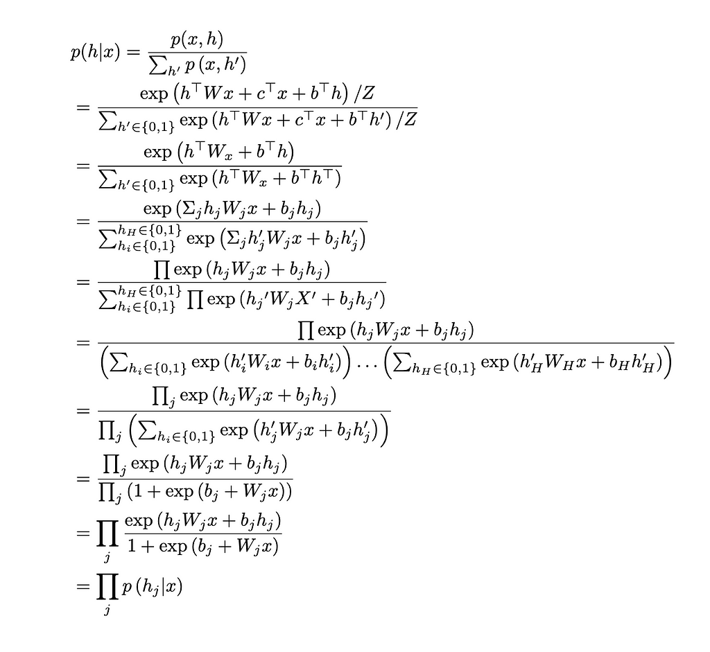
We can see the conditional distribution simplifies down to a sigmoid function where j is the jᵗʰ row of W. There is a far more rigorous calculation I have included in the appendix proving the first line of this derivation. Reach out if interested! Let’s now observe the conditional distribution p(h|x):
We can see this conditional distribution also simplifies down to a sigmoid function where k is the kᵗʰ row of W. Because of the restricted criteria in the RBM, the conditional distributions simplify to easy computations for Gibbs Sampling during inference. Once we understand what exactly the RBM is trying to learn, we will implement this in PyTorch.
Model Learning
As with most of deep learning, we are trying to minimize the negative log-likelihood (NLL) to train our model. For the RBM:
Taking the derivative of this yields:
The first term on the left-hand side of the equation is called positive phase because it pushes the model to lower the energy of real data. This term involves taking the expectation over hidden units h given the actual training data x. Positive phase is easy to compute because we have the actual training data xᵗ and can compute expectations over h due to the conditional independence.
The second term is called negative phase because it raises the energy of configurations the model currently thinks are likely. This term involves taking the expectation over both x and h under the model’s current distribution. It is hard to compute because we need to sample from the model’s full joint distribution P(x,h) (doing this requires Markov chains which would be inefficient to do repeatedly in training). The other alternative requires computing Z which we already deemed to be unfeasible. To solve this problem of calculating negative phase, we use contrastive divergence.
Contrastive Divergence
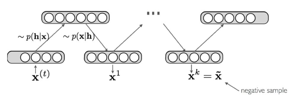
The key idea behind contrastive divergence is to use truncated Gibbs Sampling to obtain a point estimate after k iterations. We can replace the expectation negative phase with this point estimate.
Typically k = 1, but the bigger k is, the less biased the estimate of the gradient will be. I will not show the derivation for the different partials with respect to the negative phase (for weight/bias updates), but it can be derived by taking the partial derivative of E(x,h) with respect to the variables. There is a concept of persistent contrastive divergence where instead of initializing the chain to xᵗ, we initialize the chain to the negative sample of the last iteration. However, I will not go into depth on that either as normal contrastive divergence works sufficiently.
Implementing an RBM
Creating an RBM from scratch involves combining all the concepts we have discussed into one class. In the __init__ constructor, we initialize the weights, bias term for the visible layer, bias term for the hidden layer, and the number of iterations for contrastive divergence. All we need is the size of the input data, the size of the hidden variable, and k.
We also need to define a Bernoulli distribution to sample from. The Bernoulli distribution is clamped to prevent an exploding gradient during training. Both of these distributions are used in the forward pass (contrastive divergence).
class RBM(nn.Module):
    """Restricted Boltzmann Machine template."""

    def __init__(self, D: int, F: int, k: int):
        """Creates an instance RBM module.

            Args:
                D: Size of the input data.
                F: Size of the hidden variable.
                k: Number of MCMC iterations for negative sampling.

        The function initializes the weight (W) and biases (c & b).
        """
        super().__init__()
        self.W = nn.Parameter(torch.randn(F, D) * 1e-2) # Initialized from Normal(mean=0.0, variance=1e-4)
        self.c = nn.Parameter(torch.zeros(D)) # Initialized as 0.0
        self.b = nn.Parameter(torch.zeros(F)) # Initilaized as 0.0
        self.k = k

    def sample(self, p):
        """Sample from a bernoulli distribution defined by a given parameter."""
        p = torch.clamp(p, 0, 1)
        return torch.bernoulli(p)
The next methods to build out the RBM class are the conditional distributions. We derived both of these conditionals earlier:
def P_h_x(self, x):
    """Stable conditional probability calculation"""
    linear = torch.sigmoid(F.linear(x, self.W, self.b))
    return linear

def P_x_h(self, h):
    """Stable visible unit activation"""
    return self.c + torch.matmul(h, self.W)
The final methods entail the implementation of the forward pass and the free energy function. The energy function represents an effective energy for visible units after summing out all possible hidden unit configurations. The forward function is classic contrastive divergence for Gibbs Sampling. We initialize x_negative, then for k iterations: obtain h_k from P_h_x and x_negative, sample h_k from a Bernoulli, obtain x_k from P_x_h and h_k, and then obtain a new x_negative.
def free_energy(self, x):
    """Numerically stable free energy calculation"""
    visible = torch.sum(x * self.c, dim=1)
    linear = F.linear(x, self.W, self.b)
    hidden = torch.sum(torch.log(1 + torch.exp(linear)), dim=1)
    return -visible - hidden

def forward(self, x):
    """Contrastive divergence forward pass"""
    x_negative = x.clone()

    for _ in range(self.k):
        h_k = self.P_h_x(x_negative)
        h_k = self.sample(h_k)
        x_k = self.P_x_h(h_k)
        x_negative = self.sample(x_k)

    return x_negative, x_k
Hopefully this provided a basis into the theory behind RBMs as well as a basic coding implementation class that can be used to train an RBM. With any code or further derviations, feel free to reach out for more information!
Appendix
Derivation for overall p(h|x) being the product of each individual conditional distribution:

References:
[1] Montufar, Guido. “Restricted Boltzmann Machines: Introduction and Review.” arXiv:1806.07066v1 (June 2018).
[2] https://en.wikipedia.org/wiki/Gibbs_sampling
[3] Hinton, Geoffrey. “Training Products of Experts by Minimizing Contrastive Divergence.” Neural Computation (2002).
A Derivation and Application of Restricted Boltzmann Machines (2024 Nobel Prize) was originally published in Towards Data Science on Medium, where people are continuing the conversation by highlighting and responding to this story.


 Editor-Admin


